Neural networks in simple terms
Hello!
You can find various explanations of how neural networks work on the Internet, but those that I came across were either too specific and aimed at specialists, or too simplified.
I tried to write my own explanations that would not be too simplified, but at the same time as clear as possible.
The article is 10 percent compiled from other articles, 30 percent compiled from many dialogues with different LLMs, and 60 percent “handwritten” based on articles and responses.
Input data
At the input, the neural network receives incoming data in the form of a user request. General information is also added to the user's request, which allows for a more accurate answer. If the neural network supports RAG (Retrieval-Augmented Generation), then the following are also added to the request:
-
Data from the vector database, if it was previously added what is needed to generate a more relevant response
-
Extracted from an Internet page or document - in order to reduce their size, a specialized embedding neural network is often used, it finds all the appropriate pieces of text and adds them to the context of the request
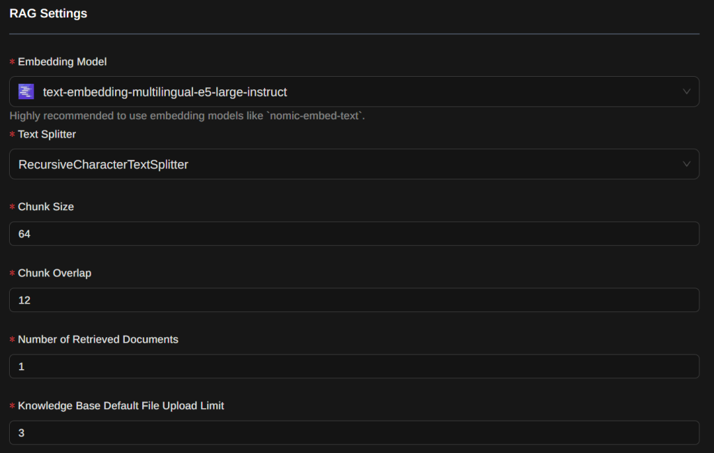
Example of neural network embedding settings for the Page Assist Chrome extension
How RAG works
The system consists of two main components
Retrieval:
Searches for relevant information from an external knowledge base (usually a vector base, such as FAISS, Qdrant, Weaviate). This base is usually built in advance from text documents (pdf, markdown, html, etc.) transformed into embeddings using a model (e.g. BERT, Instructor, or SentenceTransformer).
Generation:
LLM (GPT, LLaMA, Mistral, etc.) receives the original query + the documents found and generates the final response.
Do not confuse the two different “embeddings” in this article: here we are talking about a separate embedding model that turns a whole fragment of text into a single vector in order to find similar fragments; later, in step 2, we talk about token embeddings — the vectors of individual tokens inside the LLM itself. The mechanics are similar, but these are different models and different vectors.
I have a separate article about RAG and function calling:
And a separate one about vector databases:
Some neural networks use markup to separate the user's query, the context obtained using RAG, and the general message.
Example:
context:
this is data obtained from the Internet using an embedding neural network or from a vector storage and sorted by score matches in descending order
{"context": ["Penicillin is the first antibiotic discovered, produced from a mold fungus of the genus Penicillium. It is used to treat bacterial infections such as sore throat, syphilis, and pneumonia. Penicillin destroys the cell wall of bacteria, causing them to die.","Some people are allergic to penicillin. This can cause serious reactions, including anaphylaxis, so it is important to check for allergies before prescribing the drug."],"instructions": "Answer in simple terms, using only information from the context. If there is no answer, write 'Information not found'.","question": "What is penicillin and what is it used for?"}What the model is made of
Transformer
The neural network architecture that became the basis for modern language models such as ChatGPT, BERT, LLaMA, Gemma and many others.
It was first described in a 2017 scientific paper called “Attention is All You Need”.
Simply put, a transformer is a “smart machine” that can read and understand text by processing all words at once, rather than one at a time, as previous models (e.g. RNN, LSTM) did.
Transformer Layers
these are repeating blocks that each token within the model passes through.
One layer (or “transformer block”) includes:
*Self-Attention:* a token “looks” at other tokens and decides who is important.
Feed-Forward Network:
refining and transforming each token.
Layer Normalization or LayerNorm:
stabilizing computation.
Residual Connections:
so that the model does not “forget” the initial information.
LayerNorm can be before or after Residual (Pre-LN vs Post-LN). Virtually all modern LLMs (Llama, Qwen, Gemma, DeepSeek) use Pre-LN, and instead of classic LayerNorm — its simplified variant RMSNorm. The steps later in this article follow the classic Post-LN scheme, as it is easier to illustrate.
and other stages.
Each layer of the transformer (Transformer Block) is a separate set of parameters that:
are independently trained,
are independently applied to the input data,
provide an increasingly “deeper” understanding of the meaning and context.
What does “32 layers” mean:
each token goes through 32 such operations, one after another, after each layer the token becomes more and more informed, i.e. its representation (vector) reflects the context more and more deeply
Number of layers of popular open models (transformer layers, from official configs, as of mid-2026):
| Model | Number of layers ||---------------------------|------------------|| Llama 3.1 (8B) | 32 || Llama 3.1 (70B) | 80 || Llama 4 Scout (109B) | 48 || Gemma 3 (12B) | 48 || Gemma 3 (27B) | 62 || Gemma 4 (31B) | 60 || Qwen 3 (8B) | 36 || Qwen 3 (32B) | 64 || Qwen 3 (235B-A22B) | 94 || Qwen 3.5 (9B) | 32 || DeepSeek V3 / R1 / V4 Pro | 61 || DeepSeek V4 Flash | 43 || GPT-OSS (20B) | 24 || GPT-OSS (120B) | 36 |In MoE models (Mixture of Experts — Llama 4, Qwen 3 235B-A22B, DeepSeek V3/V4, GPT-OSS), each layer holds a set of "experts" instead of a single FFN block, and only a small part of them is activated for each token: in Qwen 3 235B-A22B, out of 235 billion parameters, only 22 billion work per token.
Activation
these are the intermediate outputs of the neural network after applying functions and layers.
We can say that activations are data that “live inside the network” at each stage of the input passing through model.
Tensor
in a neural network, this is a multidimensional array of numbers that the model layers work with.
Input data:
Text → tokens → embeddings → tensor batch_size × seq_len × embedding_dim.
Model weights:
The weight matrices in the layers are also tensors.
Intermediate representations (activations):
The output of each layer (e.g. LayerNorm, Attention) is a tensor.
Gradients:
During training, the model calculates gradients (tensors) to update the weights.
Steps of the neural network
Step 1: Tokenization (from text to tokens)
LLM doesn't work with words directly — it works with tokens (parts of words or characters) converted to numbers.
Example:
User text:"Hello, world"

Token ID in the model dictionary for the word:"Hello" = 1123"," = 15"world" = 345

Get an array of token IDs:["Hello", ",", "world"] = [1123, 15, 345]
How it's achieved:
An algorithm like Byte Pair Encoding (BPE), Unigram, WordPiece or SentencePiece is used.
BPE tokenizer finds the most frequent pairs of characters.
WordPiece builds tokens based on the probability of hierarchical partitions.
Often tokens are not individual words, but parts of words.
The vocabulary includes special word-boundary markers: in BPE vocabularies the space is encoded at the beginning of a token, while in WordPiece the “##” marker denotes word-continuation tokens. So no subtoken crosses the boundary of two words.
How the string is actually split depends on the algorithm: WordPiece is “greedy” — it takes the longest token matching the beginning of the remaining string, BPE sequentially applies the learned pair-merge rules, and Unigram picks the most probable segmentation as a whole.
Example:
User's text:"unbelievable"
Token IDs in the model's vocabulary for parts of the word:"un" = 24"believ" = 126"able" = 36
Resulting array of token IDs:["un", "believ", "able"] = [24, 126, 36]
In a WordPiece vocabulary the same word could be split as:("un", "##believable")where "##" marks a word continuation
Different words with different meanings can share common tokens — for example, "unhappy" and "unfold" both contain the token "un":
Although "un" appears in both words, the model doesn't just look at this fragment alone — it immediately considers the surrounding tokens and the entire phrase (more on that later in the article).
First, "un" is turned into a vector — just a set of numbers describing this part of the word.
Then, the transformer (a multi-layer neural network) mixes this vector with the vectors of neighboring tokens ("happy" or "fold") and adds information about their positions in the sentence.
As a result, in the first layer, "un" in "unhappy" is already different from "un" in "unfold" because the surrounding context is different.
In other words, the shared fragment "un" is neutral on its own, and the actual meaning is formed layer by layer based on the context.
Why tokens and not words:
Smaller dictionary = saves memory.
Rare and compound words are processed better.
Allows the model to "learn" to understand the structure of words.
The vocabulary size, or “vocab_size,” determines how many unique tokens the model can handle.
A larger vocabulary = fewer word splits, but a larger embedding layer.
The word “programming” can be a single token in a model with a large vocabulary,
or it can be split into parts (“program”, “ming”) in a model with a smaller vocabulary.
A practical note for readers of this blog: Cyrillic tokenizes “more expensively” than Latin script. Tokenizers are trained mostly on English, so a Russian or Ukrainian word is usually split into more tokens than an English word of the same length. The same text in Russian takes noticeably more tokens: the context fills up faster, and in paid APIs it is literally more expensive.
Vocab sizes of popular open models (from official configs, as of mid-2026):
Model | Dictionary size |--------------------------|-----------------|Llama 2 (2023) | 32 000 |Llama 3.1 | 128 256 |Llama 4 | 202 048 |Gemma 2 | 256 128 |Gemma 3 / Gemma 4 | 262 144 |Qwen 3 | 151 936 |Qwen 3.5 | 248 320 |DeepSeek V3 / R1 / V4 | 129 280 |GPT-OSS (20B / 120B) | 201 088 |You can clearly see how vocabularies grow from generation to generation. Closed models (GPT, Claude, Gemini) do not publish their vocabulary or other architecture details.
Special tokens and the chat template
Besides tokens of ordinary text, the vocabulary contains service tokens: beginning and end of a sequence, boundaries of dialogue turns, and in newer models — markers for tool calls and reasoning blocks. The model saw them during fine-tuning and relies on them to understand whose turn is whose and when to stop.
That is why, before tokenization, a dialogue is wrapped into a chat template — the markup a given model expects, with the roles “system”, “user” and “assistant”. Simplified, it looks like this:
<|system|>You are a helpful assistant.<|end|><|user|>What is penicillin?<|end|><|assistant|>The model simply continues the text after the assistant marker, and ends the generation with its service end-of-turn token.
Every model family has its own template, and mixing them up is the most common way to “break” a local setup: the model starts answering for the user, does not stop in time, or leaks service tokens right into the text. Ready-made backends like llama.cpp and Ollama usually pick the correct template from the GGUF file metadata automatically.
Image tokenization
Unlike text tokenization (where tokens are words, subwords, symbols), in images tokens are image fragments or feature representations. The main approaches are discussed below.
For images, instead of tokens, a matrix (or tensor) of pixels is obtained immediately.
In classic convolutional networks (CNN), small image patches (e.g. 3x3 or 5x5 pixels) are slid across the image, and for each patch, a convolution with a set of filters produces a feature vector. These vectors are collected into feature maps and passed on.
In modern image transformers (Vision Transformer), the image is divided into "patches" (squares, say, 16x16 pixels), each patch is aligned into a vector and also projected through the embedding matrix into a vector representation, like a token in NLP.
The main methods of image tokenization:
Patch Embedding (splitting into patches) is a classic ViT approach:
The image is divided into a grid of square patches, for example, 16x16 pixels.
Each patch is flattened into a vector, then linearly projected onto an embedding of fixed dimension (e.g. 768).
The result is a sequence of tokens: one token per patch.
Example:
224×224 RGB image with 16×16 patches → 14×14 = 196 tokens + [CLS] token.
Each token: a vector of size 768.
CNN Feature Maps as tokens:
Convolutional networks (ResNet, ConvNext) are used to extract features.
Spatial features (feature map) can be interpreted as tokens at the output, where each grid element is a vector.
Used in the ResNet variants of CLIP and other hybrid models; continuous features of a visual encoder are also used by multimodal LLMs like LLaVA.
VQ-VAE / VQ-GAN tokenization (discrete):
The encoder converts the image into a feature map and then quantizes it into discrete tokens (indices from a dictionary).
Each token is an index into a dictionary of visual patches.
Used in the first version of DALL·E, Parti, Chameleon and other generative models.
Pros: the model works with "words" of the visual language.
Cons: loss of accuracy, unstable generation.
Segment/Region-based tokens (DETR, Region Attention):
The image is divided into semantic regions (segmentation, objects).
Each region is transformed into a token using feature aggregation.
Used in object detection and visual question answering (VQA) tasks.
Patch + Positional Encoding:
As in NLP, each patch is supplemented with positional information (absolute, relative or learnable) to preserve the spatial structure of the image.
Maximum context length
Context is the working memory of the model, the context size is the maximum number of tokens (words, characters or parts of them) that the language model can process in one request.
This is the "amount of memory" that the model can see at one time to form a response. Anything beyond this window is forgotten or not seen directly by the model.
The size of the context directly affects the model's ability to remember previous messages in the conversation.
The model does not have built-in long-term memory - it does not "remember" you as a person. It simply processes the entire previous conversation as input text (tokens) passed with each request. This is called context.
Maximum context length of popular open models (from official configs, as of mid-2026):
| Model | Maximum context length ||-------------------------|------------------------------|| Llama 3.1 | 131 072 || Llama 4 Scout | 10 000 000 || Gemma 3 | 131 072 || Gemma 4 | 262 144 || Qwen 3 | 40 960 (131 072 with YaRN) || Qwen 3.5 | 262 144 || DeepSeek V3.1 / R1 | 131 072 || DeepSeek V4 | 1 048 576 || GPT-OSS | 131 072 |Closed models are in the same range: for example, Gemini 2.5 Pro handles a context of about a million tokens.
Why long context is expensive
The price of context is double. First, attention compares every token with every other token: doubling the sequence length roughly quadruples the amount of computation. Second, for every processed token the model stores its K and V vectors in every layer (the KV cache, covered in the generation-iteration step) — on long contexts this cache takes gigabytes and can eat more memory than the weights themselves.
That is why long context comes with so many engineering workarounds: Gemma and GPT-OSS interleave full-attention layers with “sliding window” layers that only look at the nearest thousand or two tokens, and DeepSeek compresses keys and values into a compact latent vector (MLA). These are the tricks that make contexts of hundreds of thousands and millions of tokens practically possible.
Step 2: Token embedding (from token to vector)
In the LLM model, for each token ID, a Token Embedding, or array of numbers, is stored. These numbers describe what that token means, as if you were translating a word into mathematical form.
Token embedding initially has a fixed value for each token, but then gets refined as it goes through the layers.
As Token Embedding goes through multiple layers of the transformer, it becomes contextualized: it takes into account the meaning of the entire phrase. The output is a vector that contains the “meaning” of the word in context.
Vector size (Embedding Size, d_model)
The number of dimensions in token embedding is fixed for the entire model and depends on its architecture.
Example:
User text:"Hello"
Token ID in model dictionary for word:"Hello" = 1123
Token embedding for token ID 1123 = array of float values with d_model= 4096 elements:[0.034, 0.120, 0.905, ..., 0.028]Embedding size (d_model) of popular open models (from official configs, as of mid-2026):
Model | d_model |--------------------------|---------|Llama 3.1 (8B) | 4096 |Llama 3.1 (70B) | 8192 |Llama 4 Scout (109B) | 5120 |Gemma 3 (12B) | 3840 |Gemma 3 (27B) | 5376 |Gemma 4 (31B) | 5376 |Qwen 3 (8B) | 4096 |Qwen 3 (32B) | 5120 |Qwen 3 (235B-A22B) | 4096 |Qwen 3.5 (9B) | 4096 |DeepSeek V3 / R1 / V4 Pro | 7168 |DeepSeek V4 Flash | 4096 |GPT-OSS (20B / 120B) | 2880 |The number of elements of the meaning vector affects:
Higher dimensionality = more “space” for storing semantics, syntax, context.
This allows us to distinguish more subtle meanings between tokens.
The price is memory: the internal projection matrices (of size d_model × d_model) grow quadratically with d_model, while the embedding layer and activations grow linearly.
a projection matrix at d_model = 4096takes up 4 times more memory thana projection matrix at d_model = 2048The numbers these vectors and weights are made of can be stored with different precision — see the section on number formats and quantization at the end of the article.
Step 3: Positional Encoding / Embeddings
Without additional information, the phrases:
“The cat eats fish”
“Fish eats the cat”
could be perceived the same, because the set of words is the same.
To give the model a sense of order, each token (word or part of a word) is added a position vector - a set of numbers that tells the model what positions the words are in.
Token embedding + Positional Encoding / Embeddings = Total vectorThis is how classic transformers did it, and it is the clearest scheme to explain. Modern models bring the position in differently — inside the attention mechanism, by rotating vectors (RoPE, covered below in this step); their total vector is simply equal to the token embedding.
Positional Encoding / Embedding is:
A vector of the same dimension as the token (d)
Represents a position in a sequence
Can be given by a formula (sin/cos) or trainable
Combined with the token vector at the input to the model
Which type is used in models:
| Method | Model/Family | Description ||-----------------------------|------------------------------------|----------------------------------------|| Sinusoidal Encoding | Transformer | Untrained, based on sines and || | (Vaswani et al., 2017) | cosines with different frequencies ||-----------------------------|------------------------------------|----------------------------------------|| Learnable Embeddings | BERT, GPT-2/GPT-3, | Learnable position table, similar to || | OPT, ELECTRA | word embeddings ||-----------------------------|------------------------------------|----------------------------------------|| Rotary Positional Embedding | almost all modern LLMs: | Vector rotation - preserves relative || (RoPE) | Llama 2/3/4, Qwen, Gemma, | positions between tokens || | Mistral, DeepSeek, GPT-OSS | ||-----------------------------|------------------------------------|----------------------------------------|| ALiBi | BLOOM, MPT | Linear bias, added to attention score, || | | does not require storing positions ||-----------------------------|------------------------------------|----------------------------------------|| Relative Position Bias | T5, DeBERTa, Transformer-XL, | Uses offsets between tokens instead of || | Pegasus, LongT5 | absolute positions |Example:
User text:"Hello, world"

Token ID in model dictionary for word:"Hello" = 1123"," = 15"world" = 345Get array of token IDs:["Hello", ",", "world"] = [1123, 15, 345]

Token embedding from model base for:Token ID 1123 = [0.034, 0.120, 0.905, ..., 0.028]Token ID 15 = [0.022, -0.010, -0.313, ..., 0.117]Token ID 345 = [-0.102, 0.241, 0.543, ..., 0.055]

Position of word token ID in user text:[1123, 15, 345] = [position 0, position 1, position 2]

Calculate or obtain from the model base the position vector:Position vector 0 = [0.001, 0.087, -0.432, ..., 0.019]Position vector 1 = [0.005, -0.013, 0.021, ..., -0.012]Position vector 2 = [-0.003, 0.099, -0.082, ..., 0.003]

Summary vector for ID 1123:Token embedding [0.034, 0.120, 0.905, ..., 0.028] +Position vector 0 [0.001, 0.087, -0.432, ..., 0.019] =[0.035, 0.207, 0.473, ..., 0.047]similarly for other tokens
Calculating Sinusoidal Position Encoding
Sinusoidal positional encoding is used in Transformer models to provide information about the position of tokens in the input sequence. Unlike recurrent networks, Transformer does not have a built-in mechanism for taking into account the order of tokens. Therefore, it is necessary to explicitly encode information about the position of each token.
From a mathematical point of view:
pos - token position in the sequence (starting with 0)i - index of the positional encoding vector dimension (starting with 0)d_model - positional encoding vector dimension (embedding dimension)PE(pos, i) - i-th element of the positional encoding vector for position pos.10000 is a hyperparameter. It is used to scale the position and frequency of the sinusoids. Choosing this value allows the model to easily extrapolate to sequences longer than the ones it was trained on.

Then the i-th element of the position encoding vector for position pos:PE(pos, 2i) = sin(pos / 10000^(2i/d_model))PE(pos, 2i+1) = cos(pos / 10000^(2i/d_model))
The formula uses different frequencies (wavelengths) of the sinusoidal functions for different dimensions of the position encoding vector.
Even dimensions use sine, and odd dimensions use cosine. This allows the model to distinguish positions at different phases and amplitudes.
Dividing pos by 10000^(2i/d_model) reduces the frequency of the sinusoid as the dimension index i increases.
This creates slower oscillations for higher dimensions, allowing the model to distinguish positions at different scales.
Example:
pos = 0 (first token)d_model = 4 (position encoding vector dimension)

Then the position encoding vector encoding PE(0) will have dimension 4.

Let's calculate each element:

i = 0:PE(0, 0) = sin(0 / 10000^(2*0/4)) = sin(0) = 0PE(0, 1) = cos(0 / 10000^(2*0/4)) = cos(0) = 1

i = 1:PE(0, 2) = sin(0 / 10000^(2*1/4)) = sin(0) = 0PE(0, 3) = cos(0 / 10000^(2*1/4)) = cos(0) = 1

PE(0) = [0, 1, 0, 1]

Now let's calculate the positional encoding vector for pos = 1:

i = 0:PE(1, 0) = sin(1 / 10000^(2*0/4)) = sin(1) ≈ 0.8415PE(1, 1) = cos(1 / 10000^(2*0/4)) = cos(1) ≈ 0.5403

i = 1:PE(1, 2) = sin(1 / 10000^(2*1/4)) = sin(0.01) ≈ 0.01PE(1, 3) = cos(1 / 10000^(2*1/4)) = cos(0.01) ≈ 1

PE(1) = [0.8415, 0.5403, 0.01, 1]
Important:
In real Transformer models, the positional encoding is usually computed for all possible positions in the sequence in advance and stored as a table.
Then, when fed with an input sequence, the corresponding positional encoding vectors are added to the token embeddings.
The choice of the hyperparameter 10000 is empirical and can be tuned depending on the specific task.
Relative positional offsets:
Instead of encoding the absolute position of each token, some Transformer variants introduce relative positional offsets. This allows the model to directly take into account the distance (and direction) between pairs of tokens, rather than their "global" position in the sequence.
Why relative offsets are needed:
When generating or processing long texts, it is important how far apart words are, and not just their absolute indices.
Absolute embeddings do not generalize well to longer sequences than those on which the model was trained.
Relative offsets provide greater flexibility: the model learns, for example, "that there can be an action object 3 positions to the right", regardless of where this sentence is in the text.
Transformer-XL, relative positions via key offsets and queries:
In classic self-attention we calculate:score_{i,j} = (Q_i · K_j) / sqrt(d_k)

In Transformer-XL, two additional sets of embeddings are introduced:E^R[r] — embedding for the relative shift r = j - iU, V — two shift vectors

Final formula:

Q_i · E^R[j-i] - content-dependent part of attention, taking into account the relative shiftV · E^R[j-i] - content-independent part, defining the basic bias for a given offsets

score_{i,j} = (1/√d_k) * (Q_i K_j + Q_i E^R[j-i] + U K_j + V E^R[j-i])
How RoPE works
Virtually all modern LLMs use Rotary Positional Embedding (RoPE). The idea: instead of adding a position vector to the embedding at the input, the coordinates of the Q and K vectors are split into pairs, and each pair is rotated by an angle proportional to the token's position. Each pair has its own rotation “frequency”, from fast to slow — much like the sinusoid frequencies above.
What this gives:
The position is brought in inside every attention layer, not once at the input.
The dot product of two rotated vectors depends only on the difference of their positions — the model gets relative positions automatically, without separate offset tables.
The V vectors and the embeddings themselves are untouched: position matters exactly where tokens are compared.
Context-stretching tricks are also tied to RoPE. If a model was trained on 40 thousand tokens and you need 130 — the rotation frequencies are rescaled so that farther positions “fit” into the range of angles the model is used to. This is how NTK scaling and YaRN work: that “131 072 with YaRN” from the context table is not separate training on long context, but a mathematical stretching of RoPE with light fine-tuning.
Step 4: Attention, Self-Attention (Attention Vector, Q,K,V-projections) and Attention Head Splitting (Multi-Head Attention)
Now that tokens have not only “meaning” but also “position,” they go through a self-attention mechanism, where each word looks at the other words to decide which one I should pay attention to in order to better understand its meaning.
This is similar to how a person reads a sentence: they can go back to previous words with their eyes to get the context right.
Self-Attention is responsible for understanding the context — which tokens are important to each other, and allows each token to look at all the others in a balanced way sequences and determine what to look for when constructing meaning.
Softmax
This is a function that takes a vector of numbers as input and turns it into a probability distribution where all values are non-negative and sum to 1.
softmax(zᵢ) = exp(zᵢ) / ∑ⱼ exp(zⱼ)
The model creates three representations for each token:
Q (question): what am I looking for?
K (key): what can I offer?
V (value): what information do I bring?
Each word compares its Q to the K of all the other words to know which one to look at. After that, it collects the necessary information from the V words that turned out to be important.
To calculate the representations, the layer weight matrix is used - this is the learning parameter of the neural network, that is, it is initialized randomly when the model is created and is trained along with the other weights. Initially random, then it becomes "smart" due to training.
How they are trained:
During the backpropagation stage, the model compares its predictions with the correct answer (e.g. the next token) and updates Wq, Wk, Wv along the error gradient using an optimizer (e.g. Adam).
The parameters Wq, Wk, and Wv can be common or different for each head, depending on the model.
Wq (Query Projection):
Creates a “question” — what the token wants to find in other tokens.
Determines the direction of attention.
Token Q = Token X total vector * Layer weight WqWk (Key Projection):
Creates a “key” — what each token offers to the others.
Used for comparison with Q (how “similar” is Qᵢ to Kⱼ).
Token K = Token Sum Vector X * Layer Weight WkWv (Value Projection):
Creates the “information” that a token can convey if it has been noticed.
Token V = Total vector of token X * Weight of layer Wv
Attention-head:
Models also have an attention-head. Each attention-head processes the input vector in its own way, through its Q, K, V projections, and looks at different aspects of the sentence.
Each attention-head has its own point of view:
one head can track grammar (for example, subject and predicate),
another — semantic connections (for example, who acts on what),
a third — positions, context, etc.
Instead of one “point of view” — several at once.
Each head sees the entire text, but — analyzes it in its own way, through projection and attention.
Example:
In the sentence
“The boy who held the ball ran away.”
Different heads can see
Head 1: “boy” ↔ “ran away” → who performs the action
Head 2: “who” ↔ “held” → nested grammatical relation
Head 3: “ball” ↔ “held” → object of the action
Each head produces its own representation for each token, taking into account its “observations.”
*Multi-Head Attention Architecture (MHA):*
Classical self-attention implementation, as in original article “Attention is All You Need”.
What’s going on:
There are multiple heads
Each head has its own Wq, Wk, Wv
Each head analyzes the entire context in its own way
The results of all heads are combined and passed through a common Wo
Pros:
Flexible: each head “looks” at the input in its own way
Works great with large computing resources
Cons:
Very expensive in memory and speed with a large number of heads
Especially with long sequences
*Multi-Query Attention Architecture (MQA):*
An optimized version of attention used in PaLM, Falcon, StarCoder and others to reduce memory load and speed up inference.
What's going on:
One Wq per head
Only one Wk and one Wv
All heads share the same keys and values
Pros:
Less memory: K and V are stored in a single instance
Faster generation: less data is stored between steps
Cons:
Less flexibility (all heads “look at” the same K and V)
May slightly degrade quality on complex tasks
Grouped Query Attention (GQA) architecture:
a combination of the previous two approaches. GQA is what most modern models use: Llama 3/4, Qwen 3, Gemma 2/3/4, GPT-OSS.
Example:
For example, the Gemma 3 neural network architecture uses Grouped Query Attention (GQA), a compromise between the standard Multi-Head Attention (MHA) and Multi-Query Attention (MQA). In this scheme, the Wq (for queries) matrices are different for each head, while the Wk (for keys) and Wv (for values) matrices can be shared across groups of heads.
In this neural network:
Wq: Each head has its own unique Wq matrix, allowing each head to focus on different aspects of the input sequence.
Wk and Wv: Heads are divided into groups, and within each group, a common Wk and Wv matrix is used. This reduces the amount of computation and memory required to store keys and values.
In Gemma 3 27B there are 32 query heads (Wq) and 16 KV heads: the heads are divided into 16 groups of 2, and each group shares the same key and value matrices (Wk and Wv).
As a result, each of the 62 layers of the Gemma 3 model of size 27B will contain:
32 different Wq (Query Projection)
16 different Wk (Key Projection)
16 different Wv (Value Projection)
1 shared Wo (Output Projection)
1 MLP with its own weights (Feed-Forward Network)
its own normalization parameters
— and each of the 62 layers has its own set of these weights.
Number of attention heads (Q heads / KV heads) of popular open models:
| Model | Q heads / KV heads ||-------------------------|------------------------|| Llama 3.1 (8B) | 32 / 8 || Llama 3.1 (70B) | 64 / 8 || Llama 4 Scout | 40 / 8 || Gemma 3 (12B) | 16 / 8 || Gemma 3 (27B) | 32 / 16 || Gemma 4 (31B) | 32 / 16 || Qwen 3 (8B) | 32 / 8 || Qwen 3 (32B) | 64 / 8 || Qwen 3 (235B-A22B) | 64 / 4 || Qwen 3.5 (9B) | 16 / 4 || DeepSeek V3 / R1 / V4 | 128 (MLA) || GPT-OSS (20B / 120B) | 64 / 8 |Instead of classic GQA, DeepSeek uses MLA (Multi-Head Latent Attention): keys and values are compressed into a shared latent vector, so counting "KV heads" does not apply to it.
*Causal Masking:*
used in some models. When a language model (LLM) generates text, it must predict the next word based only on the previous words.
This means that a Token should not have access to the tokens that come after it.
To enforce this restriction, causal masking is used - this is a mechanism that “prohibits” attention from seeing future tokens.
How it works:
In regular self-attention, each token “looks” at all tokens in the sequence, including future ones.
This is unacceptable during generation, because it would be “cheating” — the model sees the answer in advance.
To prevent this, a mask is used when calculating attention — a special matrix called an attention mask.
For a sequence of length n, a triangular mask is created in which:
Values above the diagonal are replaced with -∞ or a large negative number.
After that, softmax is applied, and these values turn into zero attention.
Example mask (for n = 4 tokens):[ [0, -∞, -∞, -∞], [0, 0, -∞, -∞], [0, 0, 0, -∞], [0, 0, 0, 0]]

This means:Token 0 sees only itself.Token 1 sees itself and token 0.Token 2 sees itself, token 1, and token 0.Token 3 sees everything before it.
Where Causal Masking is used:
GPT, LLaMA, Mistral, Gemma and other autogenerative models necessarily use causal masking.
BERT, on the contrary, uses bidirectional attention - the token can see the entire context (including the future), because the task is different - not generation, but understanding.
Why is this important, without causal masking:
During training, the model would “peek” at the correct answer (the next token).
This will lead to poor generation when using the model in inference, when the future is unknown.
The role of position in Self-Attention:
Without Position Encoding, Self-Attention only sees the meaning of words, but not their order. With Position Encoding added, Self-Attention starts to take into account not only what is written, but also where it is:
“Boy” used to “read” → he is probably a subject
“Book” next to “read” → most likely an object
What the transformer does in the end:
Each word gets information about its position
Through self-attention, each word “asks” all the others:
“What do you mean to me in this context?”
The model adds these answers together and gets a deep understanding of the meaning of the entire phrase
Repeats this on each layer (usually 12-40 times), deepening the “understanding”
User text:"Hello, world"

Token ID from the model dictionary:"Hello" = 1123"," = 15"world" = 345Getting an array of token IDs:["Hello", ",", "world"] = [1123, 15, 345]

Token embedding from the model base:"Hello" = ID 1123 = [0.034, 0.120, 0.905, ..., 0.028]"," = ID 15 = [0.022, -0.010, -0.313, ..., 0.117]"world" = ID 345 = [-0.102, 0.241, 0.543, ..., 0.055]

Calculate or obtain the position vector from the model base:Position vector "Hello" = [0.001, 0.087, -0.432, ..., 0.019]Position vector "," = [0.005, -0.013, 0.021, ..., -0.012]Position vector "world" = [-0.003, 0.099, -0.082, ..., 0.003]

For "Hello":Token embedding [0.034, 0.120, 0.905, ..., 0.028] +Position vector [0.001, 0.087, -0.432, ..., 0.019] =Sum vector X [0.035, 0.207, 0.473, ..., 0.047]

We calculate Q, K, V for each token and for each attention head:Q = X * Wq headsK = X * Wk headsV = X * Wv headswhere X is the sum vector for the tokenWq, Wk, Wv are common and the same for all tokens in this layer,but different or partially different for each head

For example:Wq heads = [[0.1, 0.2, 0.3], [0.4, 0.5, 0.6], [0.7, 0.8, 0.9], [1.0, 1.1, 1.2]]Wk heads = [[0.12, 0.22, 0.32], [0.42, 0.52, 0.62], [0.72, 0.82, 0.92], [1.02, 1.12, 1.22]]Wv heads = [[0.11, 0.21, 0.31], [0.41, 0.51, 0.61], [0.71, 0.81, 0.91], [1.01, 1.11, 1.21]]

Then:

Q "Hello" = x * Wq = [0.035, 0.207, 0.473, 0.047] * Wq

Q[0] = 0.035 * 0.1 + 0.207 * 0.4 + 0.473 * 0.7 + 0.047 * 1.0≈ 0.0035 + 0.0828 + 0.3311 + 0.047≈ 0.4644

Q[1] = 0.035*0.2 + 0.207*0.5 + 0.473*0.8 + 0.047*1.1= 0.007 + 0.1035 + 0.3784 + 0.0517≈ 0.5406

Q[2] = 0.035*0.3 + 0.207*0.6 + 0.473*0.9 + 0.047*1.2= 0.0105 + 0.1242 + 0.4257 + 0.0564≈ 0.6168

Q = [0.4644, 0.5406, 0.6168]

we calculate similarly for "Hello":K = [0.47964, 0.55684, 0.63204]V = [0.47299, 0.54822, 0.62442]and for other tokens
*Calculating Attention Score between tokens:* At this point, we have Q, K, and V for one token and one attention head. Now we can move on to calculating attention score between tokens, for example, between “Hello” and “world”, using the formula:
In mathematical terms:
Q - matrix of QueriesK - matrix of KeysV - matrix of Valuesd_k - vector dimension

Attention(Q, K, V) = softmax((Q * Kᵀ) / √d_k + mask) * V

Q * Kᵀ - matrix multiplication of Q by the transpose of K.This calculates the "raw" attention weights between each query and each key.

√d_k - square root of the dimension of key vectors.Used for scaling to prevent softmax values from getting too large, which can lead to gradient problems.This is called Scaled Dot-Product Attention.

mask is a matrix that is used to constrain attention.In generative models, a causal mask is used - it prevents a token from "seeing ahead" when computing attention.This is critical for problems where the model predicts the next token.

softmax(...) - the softmax function is applied to the result of dividing Q ⋅ Kᵀby √d_k (and adding mask if present). This normalizes the attention weights so that they sum to 1 for each query.

Multiplying the softmax result by V yields a weighted sum of the values,where the weights are determined by the attention score.
Example:
Input:

| Token    | Q-vector                 | K-vector                 | V-vector              ||----------|--------------------------|--------------------------|-----------------------|| "Hello"  | [0.4644, 0.5406, 0.6168] | [0.4796, 0.5568, 0.6320] | [0.473, 0.548, 0.624] ||----------|--------------------------|--------------------------|-----------------------|| ","      | [0.2, 0.3, 0.1]          | [0.25, 0.35, 0.15]       | [0.12, 0.09, 0.04]    ||----------|--------------------------|--------------------------|-----------------------|| "world"  | [0.55, 0.33, 0.77]       | [0.5213, 0.5967, 0.6721] | [0.55, 0.65, 0.75]    |

For simplicity, we use the dimension d_k for Q, K = 3 (for example)

Calculation:

Hello–Hello: 0.4644*0.4796 + 0.5406*0.5568 + 0.6168*0.6320 ≈ 0.2228 + 0.3011 + 0.3899 = 0.9138Hello–",": 0.4644*0.25 + 0.5406*0.35 + 0.6168*0.15 ≈ 0.1161 + 0.1892 + 0.0925 = 0.3978Hello–world: 0.4644*0.5213 + 0.5406*0.5967 + 0.6168*0.6721 ≈ 0.2422 + 0.3225 + 0.4147 = 0.9794","–Hello: 0.2*0.4796 + 0.3*0.5568 + 0.1*0.6320 ≈ 0.0959 + 0.1670 + 0.0632 = 0.3261","–",": 0.2*0.25 + 0.3*0.35 + 0.1*0.15 = 0.05 + 0.105 + 0.015 = 0.17","–world: 0.2*0.5213 + 0.3*0.5967 + 0.1*0.6721 ≈ 0.1043 + 0.1790 + 0.0672 = 0.3505world–Hello: 0.55*0.4796 + 0.33*0.5568 + 0.77*0.6320 ≈ 0.2638 + 0.1837 + 0.4876 = 0.9351world–",": 0.55*0.25 + 0.33*0.35 + 0.77*0.15 ≈ 0.1375 + 0.1155 + 0.1155 = 0.3685world-world: 0.55*0.5213 + 0.33*0.5967 + 0.77*0.6721 ≈ 0.2867 + 0.1969 + 0.5185 = 1.0021

Divide by √d_k = √3 ≈ 1.732

| From \ To | Hello                   | ","                     | world                   ||-----------|-------------------------|-------------------------|-------------------------|| Hello     | 0.9138 / 1.732 ≈ 0.5275 | 0.3978 / 1.732 ≈ 0.2296 | 0.9794 / 1.732 ≈ 0.5652 || ","       | 0.3261 / 1.732 ≈ 0.1882 | 0.17 / 1.732 ≈ 0.0982   | 0.3505 / 1.732 ≈ 0.2023 || world     | 0.9351 / 1.732 ≈ 0.5397 | 0.3685 / 1.732 ≈ 0.2127 | 1.0021 / 1.732 ≈ 0.5786 |

Apply the exponent for "Hello":

exp(0.5275) ≈ 1.694exp(0.2296) ≈ 1.258exp(0.5652) ≈ 1.759

Sum of all exponents for "Hello":

1.694 + 1.258 + 1.759 ≈ 4.711

softmax = exp(x) / sum of all exp(x)

Softmax weight for "Hello" relative to other tokens:

| Token  | Softmax weight       || ------ | -------------------- || Hello  | 1.694 / 4.711 ≈ 0.36 || ","    | 1.258 / 4.711 ≈ 0.27 || world  | 1.759 / 4.711 ≈ 0.37 |

When "Hello" generates its representation (at the output of the attention layer), it:takes 36% of the information from itself,27% from ",",and 37% from the word "world".

Weighted summation:

Output= 0.36 ∗ V("Hello") + 0.27 ∗ V(",") + 0.37 ∗ V("world")

Coordinate 1 = 0.36∗0.473+0.27∗0.12+0.37∗0.55≈0.1703+0.0324+0.2035 ≈ 0.4062Coordinate 2 = 0.36∗0.548+0.27∗0.09+0.37∗0.65≈0.1973+0.0243+0.2405 ≈ 0.4621Coordinate 3 = 0.36∗0.624+0.27∗0.04+0.37∗0.75≈0.2246+0.0108+0.2775 ≈ 0.5129

Attention output for the token "Hello": [0.4062, 0.4621, 0.5129]
This vector is the attention output, a new representation of the token "Hello", which takes into account its context: both itself and its neighbors. These vectors are then either sent to the next attention layer or to the model output. Do not confuse it with the attention score: the score is the scalar weights from softmax (0.36, 0.27, 0.37 above), while this is the sum of the V vectors weighted by them.
Note: for simplicity, the example is calculated without the causal mask - here "Hello" also "sees" the token "world" that comes after it. In a real LLM with causal masking, a token would gather information only from itself and the previous tokens.
Comparing a token with itself is necessary because in self-attention each token “looks” at all tokens, including itself.
This is necessary in order to:
Save information about the token itself — otherwise it would be “lost” against the background of the others.
Learn to “enhance” or “suppress” yourself — for example, in some language situations the token is important in itself (for example, a personal pronoun), and sometimes its context is more important.
The attention matrix is square (n × n), and its diagonal holds exactly the self-to-self attention; with a causal mask, only its lower triangle remains.
Formally, attention is the weights by which a token aggregates information from other tokens (including itself) and w1 is the “Hello” attention to itself. If it were not counted, the “Hello” token would not participate in its own output at all.
Example:
He said he would come.
When the model processes the “he” token, it needs to:
“look” at other tokens — to understand the context,
but the “he” token itself is also important, so as not to lose information about who we are talking about.
Resources:
Wikipedia: Attention (machine learning)
Understanding Q,K,V In Transformer( Self Attention)
What is Query, Key, and Value (QKV) in the Transformer Architecture and Why Are They Used?
Step 5: Head Concatenation, Concatenated Multi-Head Attention
The previous calculations were performed for each of the attention heads, now it is necessary to combine the results. Let me remind you that the results are different due to different Wq, Wk, Wv for different heads.
From a mathematical point of view:
h - number of heads of attentiond_k - dimension of the attention output of each headHeadOutput_i - attention output vector of the i-th head.

Concatenation (Combining vectors into one vector by coordinates):

concat = [HeadOutput_1, HeadOutput_2, ..., HeadOutput_h]
Example:
Input data:

Lets assume the dimension is 6 (2 heads × 3 values)

Number of attention heads h = 2Vector dimension d_k = 3"Hello" for head 1 HeadOutput_1 = [0.4062, 0.4621, 0.5129]"Hello" for head 2 HeadOutput_2 = [0.22, 0.33, 0.44]

Calculation:

Concatenation (Combining vectors into one vector by coordinates):

concat[0] = HeadOutput_1[0] = 0.4062concat[1] = HeadOutput_1[1] = 0.4621concat[2] = HeadOutput_1[2] = 0.5129concat[3] = HeadOutput_2[0] = 0.22concat[4] = HeadOutput_2[1] = 0.33concat[5] = HeadOutput_2[2] = 0.44

concat = [0.4062, 0.4621, 0.5129, 0.22, 0.33, 0.44]
Step 6: Output Projection (Wo)
After combining the attention outputs from different heads, they are typically passed through a Dense Layer to return them to the original model dimensional space.
In terms of mathematics:
concat ∈ ℝ⁶ - input vectorWₒ ∈ ℝ⁶ˣ³ - projection weight matrixoutput ∈ ℝ³ - output vector after projection

Multiplication:output = concat • Wₒ

Detailed formula for each component of the output vector:output[0] = concat[0]*W_o[0][0] + concat[1]*W_o[1][0] + concat[2]*W_o[2][0] + concat[3]*W_o[3][0] + concat[4]*W_o[4][0] + concat[5]*W_o[5][0]

Alternatively, as a sum:output_j = ∑_{i=1}^{6} concat_i ⋅ W_o[i][j] for j = 1, 2, 3

Matrix:output = concat (1x6) ⋅ W_o (6x3) = (1x3)
Example:
Input data:Model dimension d_model = 3

This means that the projection matrix W_o will havedimension (6, 3), i.e. 6 inputs → 3 outputsW_o = [ [0.1, 0.2, 0.3], [0.0, 0.1, 0.0], [0.2, 0.0, 0.1], [0.1, 0.2, 0.2], [0.0, 0.1, 0.3], [0.3, 0.0, 0.1]]

Input vector after concat:concat = [0.4062, 0.4621, 0.5129, 0.22, 0.33, 0.44]

Calculation:

x = 0.4062*0.1 + 0.4621*0.0 + 0.5129*0.2 + 0.22*0.1 + 0.33*0.0 + 0.44*0.3= 0.04062 + 0 + 0.10258 + 0.022 + 0 + 0.132= 0.2972

y = 0.4062*0.2 + 0.4621*0.1 + 0.5129*0.0 + 0.22*0.2 + 0.33*0.1 + 0.44*0.0= 0.08124 + 0.04621 + 0 + 0.044 + 0.033 + 0= 0.2045

z = 0.4062*0.3 + 0.4621*0.0 + 0.5129*0.1 + 0.22*0.2 + 0.33*0.3 + 0.44*0.1= 0.12186 + 0 + 0.05129 + 0.044 + 0.099 + 0.044= 0.3602

Final output vector:output = [0.2972, 0.2045, 0.3602]
Step 7: Adding Residual
this is the summation of the layer's input to its output. We add the output to the input vector that was fed to the input of the block (input embedding or the output of the previous layer). In a real model, the input and output of the block have the same dimension d_model and are added element by element; in our running example the input was 4-dimensional and the output 3-dimensional, so for illustration we take the first three components of the input.
This is used to:
Preserve the original information (gradients are easier to pass back).
Avoid signal “fading” through many layers.
Make it easier to train even very deep neural networks.
Input data:

Input vectorinput = [0.035, 0.207, 0.473]

Output vectoroutput = [0.2972, 0.2045, 0.3602]

Calculation:

residual = output + input = residual = [0.3322, 0.4115, 0.8332]
Step 8: Layer Normalization
normalizes values within one feature vector, that is, by feature dimension.
Why do you need it:
Eliminates bias and large-scale differences between features.
Makes training more stable.
Accelerates neural network convergence.
Works better with small batches, unlike BatchNorm.
From a mathematical point of view:
Calculate the mean:μ = (1/n) * ∑ xₙ

Calculate the standard deviation (std):σ = sqrt((1/n) * ∑ (xₙ - μ)^2 + ε)Where ε is a small number to avoid division by zero.

Normalize each element:̂xₙ = (xₙ - μ) / σ

Optionally scale and shift (trainable parameters):yₙ = γ * ̂xₙ + β
Example:
Input data:

Take the residual output from the previous step:x = [0.3322, 0.4115, 0.8332]

Calculation:

Calculate the mean:μ = (0.3322 + 0.4115 + 0.8332) / 3 = 1.5769 / 3 ≈ 0.5256

Calculate the standard deviation:σ = sqrt(((0.3322 - 0.5256)^2 + (0.4115 - 0.5256)^2 + (0.8332 - 0.5256)^2) / 3)= sqrt((0.0374 + 0.0130 + 0.0946) / 3)= sqrt(0.0483) ≈ 0.22

Normalize:̂x₁ = (0.3322 - 0.5256) / 0.22 ≈ -0.88̂x₂ = (0.4115 - 0.5256) / 0.22 ≈ -0.52̂x₃ = (0.8332 - 0.5256) / 0.22 ≈ 1.40

If the trainable parameters are γ = 1 and β = 0, this is the result:[-0.88, -0.52, 1.40]
Step 9: FFN (Feed-Forward Network) and MLP (Multilayer Perceptron)
FFN (Feed-Forward Network):
is a transformer component that processes each word (or token) individually, without regard to other tokens.
It is applied independently to each token after the attention layer and is a two-layer neural network with a non-linear activation function.
This allows the model to capture more complex dependencies.
MLP (Multilayer Perceptron):
is a type of neural network consisting of multiple fully connected layers neurons. In the context of LLM and transformers, MLP often means the same Feed-Forward Network (FFN).
MLP = general name of the architecture,
FFN = special case of MLP used inside transformers.
In terms of mathematics:
x - input vector of dimension dW1-weight matrix of the first linear layer of dimension (d_ff × d)b1-bias of the first layer of dimension d_ffW2-weight matrix of the second linear layer of dimension (d × d_ff)b2-bias of the second layer of dimension df-activation function (e.g. ReLU or GELU)d-dimension of input/outputd_ff-dimension of the hidden layer (usually d_ff = 4 × d)

Basic formula of FFN:FFN(x) = W2 f(W1 x + b1) + b2

Stepwise decomposition:

Linear transformation, dimension z1: (d_ff × 1):z1 = W1 x + b1

Nonlinear activation, applied elementwise, dimension is preserved:z2 = f(z1)

Second linear transformation, the resulting vector is the same size as x: (d × 1):y = W2 z2 + b2
Example:
Input data:

Hidden layer dimension d = 4,Internal dimension d_ff = 8,Activation: ReLU,Input vector:x = [x[0], x[1], x[2], x[3]] = [1.0, -2.0, 0.5, 3.0]

8x4 matrix W1 =[ [1, 0, 0, 0], [0, 1, 0, 0], [0, 0, 1, 0], [0, 0, 0, 1], [1, 1, 1, 1], [1, -1, 1, -1], [0.5, 0.5, 0.5, 0.5], [-1, -1, -1, -1]]

Calculation:

y[0] = 1 * x[0] + 0 * x[1] + 0 * x[2] + 0 * x[3] = 1.0 + 0 + 0 + 0 = 1.0y[1] = 0 * x[0] + 1 * x[1] + 0 * x[2] + 0 * x[3] = 0 - 2.0 + 0 + 0 = -2.0y[2] = 0 * x[0] + 0 * x[1] + 1 * x[2] + 0 * x[3] = 0 + 0 + 0.5 + 0 = 0.5y[3] = 0 * x[0] + 0 * x[1] + 0 * x[2] + 1 * x[3] = 0 + 0 + 0 + 3.0 = 3.0y[4] = 1 * x[0] + 1 * x[1] + 1 * x[2] + 1 * x[3] = 1.0 - 2.0 + 0.5 + 3.0 = 2.5y[5] = 1 * x[0] + (-1) * x[1] + 1 * x[2] + (-1) * x[3] = 1.0 + 2.0 + 0.5 - 3.0 = 0.5y[6] = 0.5 * x[0] + 0.5 * x[1] + 0.5 * x[2] + 0.5 * x[3] = 0.5 - 1.0 + 0.25 + 1.5 = 1.25y[7] = -1 * x[0] + (-1) * x[1] + (-1) * x[2] + (-1) * x[3] = -1.0 + 2.0 - 0.5 - 3.0 = -2.5

Vector after the linear layer (before activation):y = [1.0, -2.0, 0.5, 3.0, 2.5, 0.5, 1.25, -2.5]

Applying ReLU:ReLU(y[i]) = max(0, y[i])

ReLU(y) = [1.0, 0.0, 0.5, 3.0, 2.5, 0.5, 1.25, 0.0]
In modern models the FFN is slightly more complex than described: a gated variant (SwiGLU) with three matrices is used — two prepare a “candidate” and a “gate” that are multiplied element-wise — and instead of ReLU a smooth activation (SiLU/GELU) is taken; the inner dimension is then not 4×, but about 2.7× of d_model. The essence stays the same: a couple of linear layers and a nonlinearity, applied to each token separately.
In MoE models, it is exactly the FFN that is replaced by a set of “experts”: a small router picks a few of them for each token (say, 8 out of 128), and only the chosen ones run — this is how Qwen 3 235B-A22B spends only 22 of its 235 billion parameters per token.
Step 10: Residual + LayerNorm (second normalization layer)
After FFN, the input of this block (the output of step 8 — what was fed into the FFN) is added to the result again and the vector is normalized again - this helps to preserve information and stabilize the calculations
Step 11: Feeding the block output to the next transformer block
Having received a normalized vector at the output of one transformer block, the model passes it to the input of the next block. There can be dozens of such blocks — each one adds more and more “understanding” of the context
Step 12: Final LayerNorm normalization after the last block
After the last layer, LayerNorm is applied again — this is the final touch before generating logits to smooth out the spread of values
Step 13: Logits Projection + Softmax
The normalized vector from the last layer is multiplied by the embedding matrix (or a separate linear layer) to obtain the raw scores (logits) for each token in the vocabulary. These estimates are then converted into probabilities using Softmax or directly fed into samplers for token selection.
What are logits:
"raw" values that have not yet been normalized into probabilities.
For example, if the dictionary consists of 50,000 tokens, then logits are simply 50,000 numbers, one for each token.
For each token in the sequence, the model has formed a representation (hidden state).
Now we need to convert this hidden state into logits for the dictionary - an estimate of the probability of each possible next token.
Linear Layer Transformation:
logits = hidden_state @ Wᵀ + b

hidden_state: last vector (or whole sequence - but usually last token is of interest),Wᵀ: transposed matrix of embeddings (size [vocab_size, hidden_dim]),b: bias, often omitted for economy.
some models use weight tying — Wᵀ is taken from the same layer as the input embeddings, which saves memory. This is mostly done by compact models (Gemma, smaller Qwen), while, for example, large Llama and DeepSeek keep a separate output matrix.
During generation this transformation is done only for the last position: to pick the next token you need the logits of a single, last hidden state — there is no point in computing hundreds of thousands of logits for every prompt token.
Step 14: Selecting the next token (sampling)
The resulting logits are passed through a chain of samplers: first, penalties for repetitions and temperature are applied, then filters (top-k, top-p, etc.), and finally the final sampler (mirostat, greedy selection or distribution). This token is added to the context, and the generation is repeated from step 1 until the end or the desired length is reached.
In the backend LLama.cpp you can create chains of samplers, first intermediate ones, then the chain should end with the final sampler.
The order of using samplers in llama.cpp:
1. Repeat penalties:- repeat_penalty- frequency_penalty- presence_penalty- DRY (n-gram repetition penalty)

2. Token filtering:- top_k- typical_p- top_p- min_p- XTC

3. Logit scaling:- temperature

4. Grammar restrictions:- grammar

5. Final token selection:- mirostat (v1 or v2) or- greedy / dist (random sampling)
Example from LLama.cpp (for developers):
// preparing chain parametersstruct llama_sampler_chain_params sparams = llama_sampler_chain_default_params();llama_sampler * smpl = llama_sampler_chain_init(sparams);

// intermediate samplers:llama_sampler_chain_add(smpl, llama_sampler_init_top_k (50)); // Top-Kllama_sampler_chain_add(smpl, llama_sampler_init_typical (0.95f, 1)); // Locally Typicalllama_sampler_chain_add(smpl, llama_sampler_init_top_p (0.9f, 1)); // Top-P (nucleus)llama_sampler_chain_add(smpl, llama_sampler_init_min_p (0.05f, 1)); // Min-Pllama_sampler_chain_add(smpl, llama_sampler_init_xtc (0.9f, 1.0f, 1, LLAMA_DEFAULT_SEED)); // XTCllama_sampler_chain_add(smpl, llama_sampler_init_top_n_sigma(1.5f)); // Top-nσllama_sampler_chain_add(smpl, llama_sampler_init_temp (0.7f)); //Temperaturellama_sampler_chain_add(smpl, llama_sampler_init_temp_ext (0.7f, 0.1f, 1.5f)); // Extended temp

llama_sampler_chain_add(smpl, llama_sampler_init_grammar(vocab, grammar, "root"));llama_sampler_chain_add(smpl,llama_sampler_init_grammar_lazy_patterns(vocab, grammar, "root", patterns, 2, tokens, N));

// final sampler, only 1 option from:llama_sampler_chain_add(smpl, llama_sampler_init_mirostat(32000, LLAMA_DEFAULT_SEED, 5.0f, 0.1f, 100)); // Mirostat V1llama_sampler_chain_add(smpl, llama_sampler_init_mirostat_v2(LLAMA_DEFAULT_SEED, 5.0f, 0.1f)); // Mirostat V2llama_sampler_chain_add(smpl, llama_sampler_init_greedy()); // Greedyllama_sampler_chain_add(smpl, llama_sampler_init_dist(LLAMA_DEFAULT_SEED)); // Dist

// after generation, do not forget to free the chain:llama_sampler_free(smpl);
I have a separate article about llama.cpp:
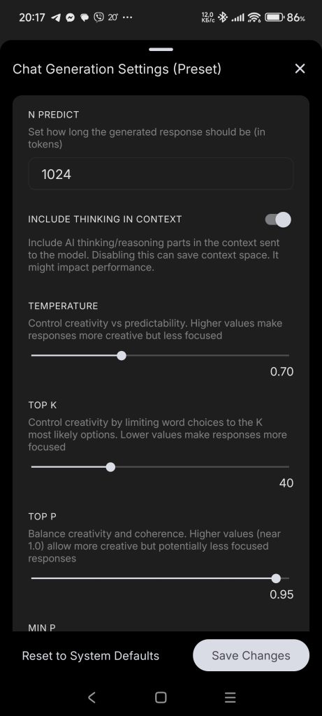
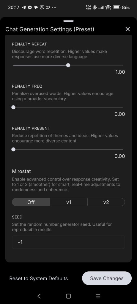
Example of the sampler settings page from the application https://github.com/a-ghorbani/pocketpal-ai
Intermediate samplers
Temperature (temp)
controls the degree of randomness in choosing the next token from the probability distribution calculated by the model. Temperature narrows or widens the "choice funnel" of the next word. The lower it is, the narrower the funnel, the higher it is, the wider it is.
After the model has predicted the logits (raw probabilities) for all possible tokens, they are passed through a softmax function. Temperature affects this function:
P(token) = softmax(logits / temperature)Effect of temperature parameter:
T = 1 logits are left as is.
T < 1 (e.g. 0.7) the model increases the differences between tokens - probable tokens become even more probable. Behavior becomes more predictable.
T > 1 (e.g. 1.5) the differences between tokens are smoothed out - the chance of choosing a less probable token increases. Behavior becomes more diverse and risky.
T → 0 softmax becomes argmax, and one most probable token is always chosen.
Initial logits:Token A: 3.0Token B: 2.5Token C: 1.0

After softmax without change (temp = 1.0):A: 57%B: 35%C: 8%

With reduced temperature (temp = 0.5):A: 72%B: 27%C: 1%

With increased temperature (temp = 1.5):A: 51%B: 36%C: 13%
Top-k
the model selects the next token only from the k most probable ones. All other tokens are discarded, regardless of their absolute probability.
there are 6 tokens with the following probabilities:A: 0.35B: 0.30C: 0.15D: 0.10E: 0.06F: 0.04

If top_k = 3, then we leave only:A: 0.35B: 0.30C: 0.15
Top-p (nucleus sampling)
the minimum set of tokens with the highest probabilities, the sum of which exceeds the specified threshold p, is selected. The remaining tokens are completely cut off, even if they had a high rank.
the model gave the token probabilities:

A: 0.50B: 0.25C: 0.15D: 0.08E: 0.02

With top_p = 0.9, we take the highest-probability tokensuntil their sum reaches the threshold:0.50 + 0.25 + 0.15 = 0.90 — A, B, C remainD and E will be discarded — then the probabilities of the rest are normalized again.
Min-p
all tokens whose probability is below a threshold defined as a fraction p of the probability of the most likely token are cut off. For example, with min_p = 0.1 and a leader probability of 0.50, the threshold is 0.05 — everything below it is discarded. The threshold is relative: when the model is confident, the filter is stricter; when the distribution is flat, it is softer.
Typical sampling
selects tokens that are close to the "typical" level of surprise, excluding those that are too predictable and too rare. Unlike top-k and top-p, it focuses on the median surprisal value rather than the probability of tokens.
Repetition penalties, Frequency penalty, Presence penalty
reduces the chances of re-selection of already generated tokens by decreasing their logits. This helps to avoid annoying repetitions in the text and makes the output more diverse.
Logit bias
a method that allows you to manually change the probability of individual tokens before applying softmax by adding or subtracting values from their logits. This gives fine-grained control: you can, for example, force the model to avoid certain words or, conversely, choose them more often.
Tail Free Sampling (TFS)
drops the long "tail" of the distribution, adjusting the probability density.
DRY (Don't Repeat Yourself)
penalizes tokens that would continue n-grams already seen in the text: the longer the resulting repetition, the stronger the penalty. It removes looping on whole phrases well, without touching single word repetitions.
Grammar
uses grammar rules (usually in the form of CFG) to strictly constrain the allowed tokens at each generation step. Instead of changing the logits, it simply disallows all tokens that do not match the current legal state of the grammar, ensuring a strictly structured output.
and others
Final samplers
Greedy
the simplest generation method, in which the model always selects the token with the highest probability (maximum logit). It is fast and deterministic, but often leads to monotonous and predictable text.
Random
the next token is chosen randomly, proportional to its probability after all samplers (top-k, top-p, etc.) have been applied. This is the opposite of greedy, which always takes the token with the highest probability.
Dist
this is what llama.cpp calls the final random sampling: the token is chosen randomly, proportional to the final probability distribution after all filters — the same as Random above, with a fixable seed for reproducibility.
Mirostat v1
maintains a given level of "surprise" (perplexity), dynamically adjusting the choice of words. It helps avoid excessive repetition (the boredom trap) and incoherence (the confusion trap), ensuring balanced and high-quality text generation.
Mirostat v2
maintains a given level of surprise (perplexity) with more precise control than Mirostat v1. It uses an advanced feedback mechanism that allows dynamic adjustment of word choice to achieve consistent text quality.
and others
Step 15. Iterate generation
After the model selected the next token, its ID is added to the end of the input sequence — no re-tokenization is needed, the selected token is already a token.
Then the loop repeats: the model computes attention taking the new token into account and predicts the next one, and so on until the termination conditions are met.
There is no need to recompute all previous tokens either: their K and V vectors are stored in the KV cache, and on each iteration only the new token is actually processed — which is why generation steps take roughly the same time.
This is where the two phases of the model's work come from, familiar to everyone as “it thinks, then types steadily”. First comes prefill: the whole prompt is processed in one parallel pass, filling the KV cache — that is the pause before the first word, and the longer the prompt, the longer it lasts. Then comes decode: tokens are generated one by one, each in roughly the same time. That is why a model's speed is described with two different numbers — time to first token and tokens per second.
This loop allows you to build the entire output sequence one token at a time.
Termination conditions
Generation ends when the model produces a special end-of-sequence (EOS) token or when a predefined maximum sequence length is reached.
This limitation prevents infinite or overly long responses.
Generation is also stopped by stop sequences: predefined strings (for example, the marker of the next dialogue turn) that cut off the output as soon as they appear.
Step 16. Converting tokens to words
Once the model has generated the required number of tokens, they are converted back into text - this is called detokenization. The tokenizer takes a sequence of numbers (tokens) and translates them into words and punctuation marks. In practice, chat interfaces do this on the go — that is what streaming is: every selected token is immediately detokenized and appended on screen, which is why the answer appears word by word instead of all at once at the end.
How the model was trained
Everything above describes an already finished model at work. The model itself is produced in several stages.
Pretraining:
The model solves one and the same task trillions of times — predict the next token in text from a huge corpus (web, books, code). No labeling is needed: the correct answer is simply the real next token. At this stage the model learns language, facts and patterns, but all it can do is continue text.
Instruction tuning (SFT, Supervised Fine-Tuning):
The model is fine-tuned on “request → good answer” examples, written by people or selected from generations. After this it answers questions instead of continuing them.
Alignment (RLHF, DPO):
People compare pairs of model answers and pick the better one; on these preferences the model is tuned to give useful and safe answers. The classic way is reinforcement learning from human feedback (RLHF); a simpler modern alternative is DPO, where the preferences are used directly as training examples.
Reasoning models
The “thinking” models from the tables above (DeepSeek R1, Qwen 3 in thinking mode, Gemma 4) are mechanically no different: the same transformers generating the same tokens. The difference is in training: they were additionally trained with reinforcement learning on tasks with verifiable answers, rewarded for the correct result — and the model taught itself to write a long chain of reasoning before the answer, a draft that the interface then hides behind a spoiler. The price is paid in tokens: a “thinking” answer can be several times longer and slower than a regular one.
Where hallucinations come from
Straight from the generation mechanics. The model must always pick a next token — it has no built-in “I don't know” state, only a probability distribution from which something will be selected. If the weights hold little knowledge about the subject, the distribution will still produce a plausible-sounding continuation: the correct form of an answer with invented content. That is why hallucinations are not a bug that will one day be fixed, but a property of the approach itself; they are suppressed by training (teaching the model to decline), by tools like RAG and web search — but never eliminated completely.
Interesting questions and answers
Is it possible to describe in a few sentences how a neural network works?
I'll try. The model is a huge function trained for a single task: given the beginning of a text, predict which token (a piece of a word) is most likely to come next. Your question is turned into a sequence of tokens, the model computes the probabilities of all possible continuations, one token is selected from them and appended to the text — and it all repeats, token by token, until an answer takes shape. All the “understanding” lies in the fact that, over training on an enormous corpus of text, the model's weights learned to predict that continuation based on the meaning and context of the whole phrase, not just word frequency.
Why do LLM models give a question as input and output an answer, rather than a rephrased question?
The model is trained on “question → answer” texts, so when a question is presented, it does not generate the words of the question itself, but the most probable continuation — the answer.
During instruction tuning (SFT) and RLHF it is "rewarded" for useful answers, not for repeating the wording, so the parameters shift towards answering.
In terms of probabilities: for a question, the probability of the next answer token is higher than the token repeating the question, and the decoder chooses it.
The data on which the LLM model is trained is becoming outdated, what are the possibilities for the model to generate relevant answers?
Retrieval-Augmented Generation (RAG):
When a query is requested, the model searches for relevant documents in the current external database (search by vector or text index) and uses their context when generating a response. This way, you can get fresh information without overtraining the main network
Parameter-efficient retraining (LoRA, Adapters):
Instead of completely retraining the model, small adapters or low-rank matrices (LoRA) are built in, which are trained on new data. This allows you to quickly and inexpensively "teach" the model new facts or domains
I made a separate article about LoRA:
Model Editing:
Algorithms like MEMIT/ROME locally adjust the model weights to add or update specific facts without affecting the rest of the knowledge
Separate knowledge bases and graphs:
Instead of storing facts inside LLM parameters, move them to external KBs or knowledge graphs that are regularly updated, and the model only queries them for information
Integration with web search and API:
Connecting the model to live sources — built-in web search in chatbots, calls to external APIs and tools (function calling, MCP servers) — directly returns fresh content.
How does the LLM model understand different languages?
The model “understands” different languages because during the training process it sees texts in many of them and learns to predict the next fragment regardless of the language. Key points:
Large multilingual corpus:
Texts (Wikipedia, books, web pages from Common Crawl, etc.) in dozens and hundreds of languages are collected for training. For example, the open BLOOM model had about 46 languages, and the share of each depends on the volume of available data
General subword tokenization:
Algorithms like BPE or SentencePiece are used, which break words into fragments (subword) and include symbols and sequences from different alphabets in the dictionary. So the model operates with a single set of tokens for all languages
Universal transformer architecture:
The same weights are used in the transformer when processing any language. Therefore, when training in different languages, the model finds common patterns (syntax, semantics) and uses cross-lingual transfer of knowledge
Not all languages and not in all volumes:
They train only in those languages where there is a sufficient volume of texts. Rare or low-resource languages are included in separate pretraining or receive a smaller share of data, so the quality of generation on them is lower
Special pretraining and adapters:
To improve knowledge of little-known languages, continuous pretraining is used on local data or adapters (LoRA) are inserted, which fine-tune the model's knowledge for a specific language.
Additional information
Vector precision
Also, the floating-point numbers that make up the vector can have different precision:
Lower precision reduces the size of the model and speeds up processing.
Usually, models are trained at full FP32 precision (float32), that is, the vector consists of 32-bit numbers.
Quantization
Quantization is used to reduce precision and make the model lighter — the process of converting floating-point numbers (e.g. FP32) into more compact integer representations (e.g. INT8), while preserving the approximate value.
This introduces a small loss of precision, but it often does not critically affect the output quality.
Format: FP32 (float32), 32 bits = 4 bytesPurpose: Full precision. Used for training models, as well as for precise inference.Provides maximum precision, but requires a lot of memory and computing resources.Binary value: 01000000 01001001 00001111 11011011Actual value: 3.14159Possible quantization types: Not used - this is the full (not quantized) format.

Format: FP16 (float16), 16 bits = 2 bytesPurpose: Half precision. Used for accelerated training and inference on GPUs (e.g. NVIDIA Tensor Cores).Faster and 2x more memory efficient than FP32.Binary value: 01000010 01001000Actual value: ≈ 3.140625In GGUF files, unquantized weights of this precision are labeled F16.

Format: BF16 (bfloat16), 16 bits = 2 bytesPurpose: Alternative to FP16, used in TPU and some GPUs. Has the same exponent as FP32, but a shortened mantissa.Faster and more compact, while maintaining the range of FP32.Binary value: 01000000 01001001(these are simply the first two bytes of the FP32 representation — the mantissa is truncated)Actual value: ≈ 3.140625In GGUF files it is labeled BF16.

Format: INT8 (8 bits), scale = 0.125Purpose: Quantized integer. Used in optimized models for inference on CPU and mobile devices.Requires scale and offset (zero_point) restoration.Quantized value: 25Binary value: 00011001Actual value: 25 × 0.125 = 3.125Possible quantization types: Q8_0, Q8_1, Int8Affine, PerChannelQuant (ONNX), dynamic/int8 (TensorFlow Lite)

Format: INT4 (Q4), 4 bits, scale = 0.5 (2 numbers in 1 byte)Purpose: Very compressed format for language models. Used in llama.cpp, GGUF and other systems.Provides significant reduction in model size. Requires reconstruction (dequantization) at startup.Quantized value: 7 (maximum value for signed 4-bit int: -8…+7)Binary value: 0111Actual value: 7 × 0.5 = 3.5Possible quantization types: Q4_0, Q4_1, Q4_K_S, Q4_K_M (llama.cpp, GGUF)

Format: INT2 (Q2), 2 bits, scale = 1.0 (4 numbers in 1 byte)Purpose: Extremely compressed format for use in LLM on devices with limited resources.Used in some variants of GGUF, MLC, and in experiments with extreme quantization.Quantized value: 1 (maximum values: -2…+1)Binary value: 01Actual value: 1 × 1.0 = 1.0Possible quantization types: Q2_K (llama.cpp, GGUF)The real Q2_K also stores per-block scales, so it actually spends about 2.6 bits per weight.

Format: INT1 (Q1), 1 bit, scale = 2.0 (8 numbers in 1 byte)Purpose: Minimum possible precision. Used in binary neural networks and prototypes.Usually values are -1 or +1. Rarely used in LLM, but can be useful in BNN (Binary Neural Networks).Quantized value: 1Binary value: 1Actual value: 1 × 2.0 = 2.0Possible quantization types: BinaryNet, XNOR-Net (usually in academic/experimental BNNs)A modern example of extreme LLM quantization is BitNet b1.58 with ternary weights -1/0/+1 (~1.58 bits per weight).
Models can also have additional quantization parameters:
_K- Denotes "K-Block" quantization.- Weights are split into blocks of fixed length (e.g. 32 or 64 values).- Within each block, a common scale and zero_point are used.- This allows for a significant reduction in model size while maintaining higher accuracy compared to simple quantization.- Example formats: Q2_K, Q4_K, Q6_K, Q8_K

_0, _1- Indicate which quantization scheme is used:- _0: basic scheme, no bias, one scale per block- _1: improved scheme, with additional bias or scale shifts- Used in formats: Q4_0, Q4_1, Q5_0, Q5_1, Q8_0, Q8_1- As a rule, _1 provides better accuracy with a slight increase in size

Size variant labels: K_S, K_M, K_L

K_S- Small — the smallest and most aggressively compressed variant- Maximum memory savings at the expense of quality

K_M- Medium — a middle trade-off between accuracy and size- The most popular choice for local use

K_L- Large — the largest and most accurate of the K variants- Slightly more memory, slightly higher quality

Example of the model name:"mistral-7b.Q4_K_M.gguf" — this means:- Mistral 7B model- Q4_K (4-bit K-block) quantization is used- Size variant: Medium

Besides K-quants, llama.cpp also has newer I-quants(IQ2_XXS, IQ3_S, IQ4_XS, etc.) — they offer better qualityat the same size thanks to a more complex encoding scheme.
Product Quantization
A method that allows you to strongly compress feature vectors (embeddings) by breaking them into parts and encoding each part through the closest template (cluster). It is used in vector databases and nearest-neighbor search (e.g. FAISS); LLM weights themselves are usually not compressed with it.
How it works:
There is a vector (for example, 128 numbers in size). This can be a text or image embedding from a neural network.
We break the vector into pieces - for example, 8 parts with 16 numbers (128 / 8 = 16).
For each position of the piece, we train our own encoder (quantizer) - on big data, we select in advance which "templates" (cluster centers) are similar to possible pieces.
For example:
the first piece can be similar to template #12,
the second - to template #3,
the third - to template #88,
and so on.
We save only the numbers of these templates. Instead of storing 128 numbers (float32 = 512 bytes), we store, for example, 8 numbers (1 byte per pattern) - 8 bytes in total.
*QAT (Quantization-Aware Training) quantization:* is a method of quantization of neural networks, in which quantization is taken into account already during model training. It allows to achieve almost the same accuracy as the original model with float parameters, while the model will use more compact int8 or other low-bit formats suitable for efficient execution on devices with limited resources (for example, smartphones or microcontrollers).
How QAT works - step by step:
Model in float32:
Training starts with a regular model using floating-point numbers (usually float32). This ensures high accuracy and stability of training.
Quantization imitation during forward pass (fake quantization):
At each forward pass, the values (weights, activations) are emulated as quantized, i.e. they are converted to int8 and then back to float32. This allows the model to "see" quantization errors already at the training stage.
float32 → int8 → float32
Thus, during backpropagation, gradients are calculated using the float32 version, but errors due to quantization still affect training.
Backward pass:
Gradients are calculated as usual, but taking into account distortions from fake quantization. This allows the model to adapt to the fact that the weights and activations will be used in low precision later.
Exporting the final model to int8:
Once training is complete, the weights are indeed quantized to int8, and the model can be compiled and run in production.
What exactly is quantized:
Weights are float32 → int8
Activations are float32 → int8
(Sometimes gradients and intermediate states are also quantized, but this is rare.)
Why use QAT:
Higher accuracy than post-training quantization (PTQ)
Low memory consumption
Faster execution on CPU/GPU/NPUs with int8 support
Especially important for mobile and embedded devices (e.g. Android)
How much memory a model needs
A rough formula: number of parameters × bytes per weight, plus the KV cache, plus a little for activations.
7-8B model:FP16 (2 bytes per weight)   ≈ 14-16 GBQ8 (1 byte per weight)      ≈ 7-8 GBQ4 (~0.6 bytes per weight)  ≈ 4-5 GB
27-32B model in Q4          ≈ 16-20 GB70B model in Q4             ≈ 40+ GB
Plus the KV cache: depends on context length,at tens of thousands of tokens — several more GB.
A practical rule for local use: look not at the “billions of parameters” but at the size of the specific GGUF file — it honestly shows how much memory the weights will take — and leave headroom for the context.
Launch methods (backends) for LLM models
vLLM:
The main server-side LLM inference engine: continuous batching of requests and PagedAttention for an economical KV cache; the de facto standard for deploying open models on GPUs.
Formats: Hugging Face weights (.safetensors)
SGLang:
A fast-growing alternative to vLLM with KV-cache reuse across requests (RadixAttention); strong at structured generation and agent workloads.
Formats: Hugging Face weights (.safetensors)
NVIDIA TensorRT-LLM:
A specialized LLM layer on top of TensorRT: compiles the model for specific NVIDIA GPUs, maximum speed at the cost of flexibility.
Format: compiled engine
ONNX Runtime:
Cross-platform engine for running ONNX models.
File format: .onnx
TensorFlow (Inference API):
Standard engine for TensorFlow models, supports SavedModel and frozen graph.
Formats: SavedModel folder (saved_model.pb + variables/), single .pb file
LiteRT (formerly TensorFlow Lite):
Lightweight engine for mobile and embedded devices, optimized for size and speed.
Format: .tflite
PyTorch (TorchScript):
Allows you to serialize and run models without depending on Python, with JIT optimizations.
Formats: .pt, .pth
NVIDIA TensorRT:
Hardware-accelerated engine for NVIDIA GPUs, compiles models (usually from ONNX) for a specific card.
Format: compiled engine .engine (or UFF/ONNX plan → .engine)
Intel OpenVINO:
Optimizes and accelerates networks on CPU and Intel GPU/VPU, converts models to IR format.
Formats: .xml (structure) + .bin (weights)
Apple Core ML:
Framework for running models on iOS/macOS, integrates with Xcode and is accelerated via Core ML Runtime.
Formats: .mlpackage, legacy .mlmodel
Microsoft ML.NET:
.NET engine for inference on CPU, suitable for C# and F#.
Format: model archive .zip
Apache TVM:
Compiles and optimizes models for various hardware, creates native libraries.
Formats: serialized Relay module or compiled library (.so, .dll)
Alibaba MNN:
Mobile neural engine with extensive optimizations for ARM, supports server launch.
Format: .mnn
Tencent NCNN:
Compact engine for mobile CPU/GPU, no third-party dependencies.
Formats:.param (structure) + .bin (weights)
OpenCV DNN:
Computer vision module with support for various formats (ONNX, Caffe, TensorFlow, Darknet).
Formats: depends on the source — .onnx, .pb, .caffemodel + .prototxt, .weights
Unity Sentis (formerly Barracuda):
Engine for running neural networks in Unity games, supports ONNX models.
Formats: .onnx, .sentis
MLC LLM:
ML compiler and engine for LLM, compiles weights into its IR and shards them.
Format: …-MLC directory with .bin shards and JSON configs (e.g. mlc-chat-config.json)
MediaPipe:
A framework for creating multimodal pipelines (detection, segmentation, etc.), based on TFLite.
Formats: .tflite (model) + .pbtxt (graph)
llama.cpp:
C++ engine for LLaMA-like models with CPU/GPU quantization support.
Format: .gguf (the old GGML .bin format is obsolete)
GGML:
Library for efficient model inference (the basis of llama.cpp and others).
Formats: .gguf, .bin
NeuralMagic DeepSparse:
Optimized engine for sparse neural networks on CPU.
Format: .onnx
AWS Neuron SDK:
An engine for accelerating inference on AWS Inferentia, compiles models for Neuron.
Formats: Neuron artifacts (.nef or library)
The following engines are mostly historical: you will hardly meet them today, but they appear in older materials.
Glow:
Facebook compiler and runtime for neural networks, ONNX input format.
Formats: intermediate .bc file or compiled .so library
Apache MXNet:
Framework with its own runtime for CPU/GPU, supports Docker deployment.
Formats: .params (weights) + .json (network)
Caffe:
Classic engine for CV networks, often used in research.
Formats: .caffemodel (weights) + .prototxt (network description)
Applications for running LLM models
LM Studio:
Desktop application for Windows, macOS and Linux with GUI for running local LLM (GPT-like).
Model formats: .gguf, .bin
Ollama:
Lightweight CLI/GUI client for Windows, macOS and Linux, works out of the box with LLM.
Model formats: .gguf, .bin
Jan:
An open desktop client for Windows, macOS and Linux in the spirit of LM Studio, but fully open source; runs on top of llama.cpp.
Model formats: .gguf
Open WebUI:
A web interface for Ollama and any OpenAI-compatible servers: chats, RAG over your own documents, multiple users; installs locally or on your own server.
Model formats: whatever the connected backend supports
KoboldCpp:
A single-file build of llama.cpp with a web interface and rich sampler settings, popular for creative writing.
Model formats: .gguf
llama.cpp (prebuilt binaries):
Ready-made executables for Windows/macOS/Linux, allow you to run LLaMA-like models without installing dependencies.
Model formats: .bin, .gguf
A separate group — applications for image generation (Stable Diffusion), not LLM:
Automatic1111 Stable Diffusion WebUI:
The most popular local web interface for generating images on Windows/macOS/Linux.
Model formats: .ckpt, .safetensors
DiffusionBee:
Desktop application for macOS (there are beta builds for Windows), "all in one" for Stable Diffusion.
Model formats: .ckpt, .safetensors
InvokeAI:
Cross-platform package with CLI and WebUI for generating images based on Stable Diffusion.
Model formats: .ckpt, .safetensors
LLM models storage format
.pt / .pth
Used in PyTorch to save trained models
Stores weights and model structure (or just weights).
Based on Python serialization (pickle), which makes them not very safe.
Suitable for training and retraining.
Not optimized for mobile inference or external inference
Can be memory intensive (FP32).
.safetensors
An alternative to .pt, a safe and fast format for PyTorch.
Does not use pickle, which means it is safe to load.
Supports parallel loading, which speeds up work.
Only for storing weights (structure is separate).
Suitable for inference and retraining.
Supports HuggingFace, PyTorch, JAX.
.bin
A general-purpose or proprietary binary format for model weights, especially in HuggingFace and old GGML.
Can be unformalized (structure depends on framework).
Can contain full weights or quantized data.
Suitable for loading into custom engines (e.g. llama.cpp).
Requires precise knowledge of how to interpret the contents.
Often used in legacy projects or custom pipelines.
.gguf
The GGML ecosystem standard for running LLM in llama.cpp, Ollama, LM Studio.
Includes everything in one file: weights, dictionary, tokenizer, model parameters.
Supports different types of quantization (Q2_K, Q4_0, Q8_1, etc.).
Well compressed and optimized for running on CPU, GPU, Android.
Fast loading and easy to process by C++ code.
The main choice for local LLM running (Gemma, LLaMA, Mistral).
.onnx
Cross-framework format for running models in different environments (Windows, Web, C#, Java, etc.).
Standardized, supported by many frameworks (PyTorch, TF, Keras).
Simplifies the transfer of models between platforms.
Suitable for inference (not for training).
Optimized by ONNX Runtime (compression, quantization).
An excellent choice for running models in embedded environments and .NET.
.tflite
Format for running TensorFlow models on mobile devices (Android, iOS).
Very compact and fast.
Supports INT8 and FP16 quantization.
Works with the LiteRT (formerly TensorFlow Lite) interpreter, easily integrated into Android.
Cannot train or retrain - only run.
Originally aimed at compact CNN/RNN models, but nowadays small LLMs (e.g. Gemma) also run on it via LiteRT and MediaPipe LLM Inference.
MLC LLM format
Running LLM on Android/iOS/GPU via compilation; there is no single container file — the model is stored as a directory with weight shards and JSON configs plus a library compiled for the device.
The model is pre-compiled into efficient bytecode.
Supports Vulkan/Metal/OpenCL for acceleration.
Used for Gemma, Mistral, LLaMA on phone.
Requires complex preparation (TVM, scripts, setup).
Great for mobile applications without servers.